Sirius Tutorial 2: Working with protein structures

Step 1

Open Sirius application window. Follow instructions from Step 1 of the first tutorial to check which directory is set as default and what zoom mode is currently set.

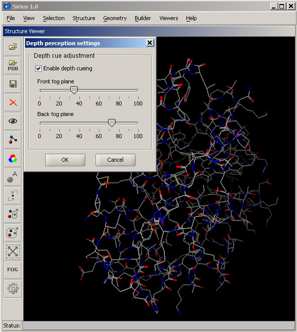
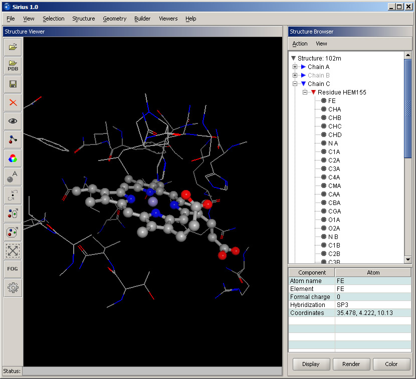
For illustration purposes, we will use a structure of hemoglobin. Click the PDB button in the toolbar or select Load from PDB option in the File menu. Then enter 102m and click OK. The structure of the protein colored by element will load in the 3D workspace. By default, atoms are not shown, since bonds alone provide a good representation of the structure. In addition, protein structures contain thousands of atoms, and rendering them would make the application too slow. It is possible to render any number of atoms, but it is recommended that this option be used only to make illustrations.

In order to improve the feeling of depth, a "fog" is simulated in the viewer. You can adjust it to achieve the best possible effect by opening the fog dialog - use Set depth perception option in the View menu or the FOG button in the toolbar. The top slider indicates where the fog starts, and the bottom slider represents where it ends and the structure completely disappears from the view. Ideally, the front fog boundary should be right before the structure, and the back boundary should be immediately behind it. You may adjust the sliders until you get the best feel for the structure depth.

Step 2

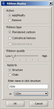
In order to display secondary structure of proteins, ribbon diagrams are used. Select Protein ribbon display from the View menu. With the default settings, specify what structure the ribbon should be created for. In the Apply to panel, leave Structure selected and choose the loaded protein (102m) from the pulldown menu.

At this point, leave the quality setting at the lowest level, since with a ribbon created at this level any selection and coloring events will be the fastest. Higher quality levels produce a much more smooth and shiny surface of the ribbon, but they make selection and coloring events much slower. Therefore, they should be used only for making illustrations. Click OK, and the ribbon cartoon will appear.

If you need to modify an existing ribbon (change quality or switch to cylindrical helices), you can use the same dialog.

Once the ribbon is displayed, open Protein ribbon color from the View menu, select 102m in the pulldown menu in the Apply to panel and choose any color form the panel on the right. Then click OK.

Since the default setting is to color the atomic structure together with the ribbon, the entire structure will change color. The display should look similar to the screenshot below.

Note: The term Structure used in various dialogs normally applies to the atomic structure, while Ribbon refers to the ribbon cartoon.

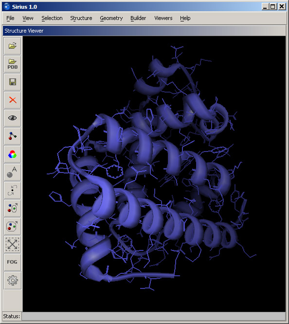
Select Color option from the View menu, select 102m from the structure list and leave the default option Color by element. This will return the default colors of the protein structure.

Step 3

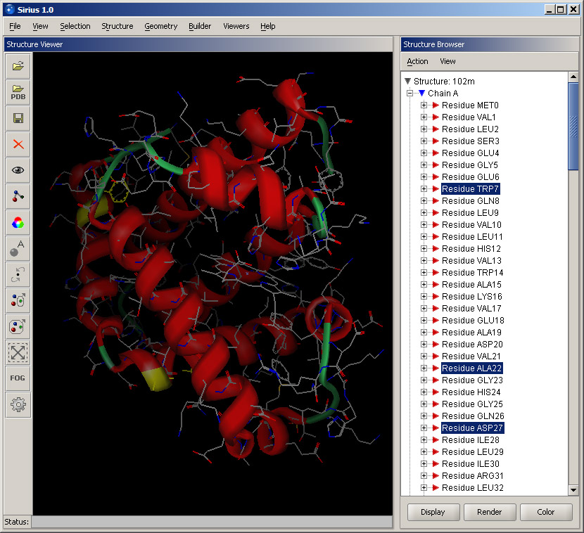
Open Structure Browser by selecting the corresponding option in the Viewers menu. This will open another panel within the Sirius windows. It lists the loaded structures (in this case, 102m) and their chains. Chains are marked with their identification names, as they appear in the PDB files. Double-click Chain A or click the + sign next to it. The tree branch will expand and show all residues present in this chain. Since this is the main protein chain, it has a large number of residues displayed in the order they appear in the protein. Click some residues in the Structure Browser and notice that the corresponding parts of the structure are highlighted. You can add residues to selection by holding the Control key. Selection in the Structure Browser can be cleared by either clicking anywhere within the 3D window or by choosing Clear selection option in the Action menu of the Structure Browser.

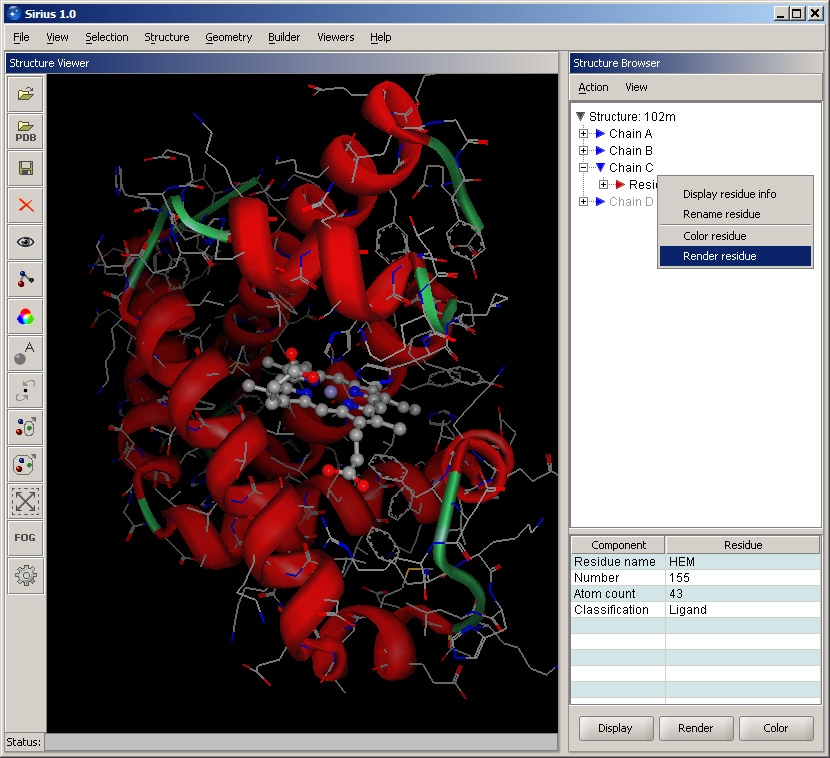
Collapse the Chain A list by clicking the "-" sign next to it, and expand Chain C instead. It contains only one residue, and that it the molecule bound to the protein - the heme. While keeping the mouse on the residue (HEM155), right click. A shortcut menu is displayed with some basic options. Select Display residue info. This will open a small panel in the lower part of the Structure Browser with some information about the residue. It shows its name, number, atom count and classification (in this case, it's a ligand). Bring up the shortcut menu again by right-clicking and select Render residue. In the displayed dialog, select Ball and stick and set quality at Best. Then click OK. The heme will become rendered and much more visible within the structure.

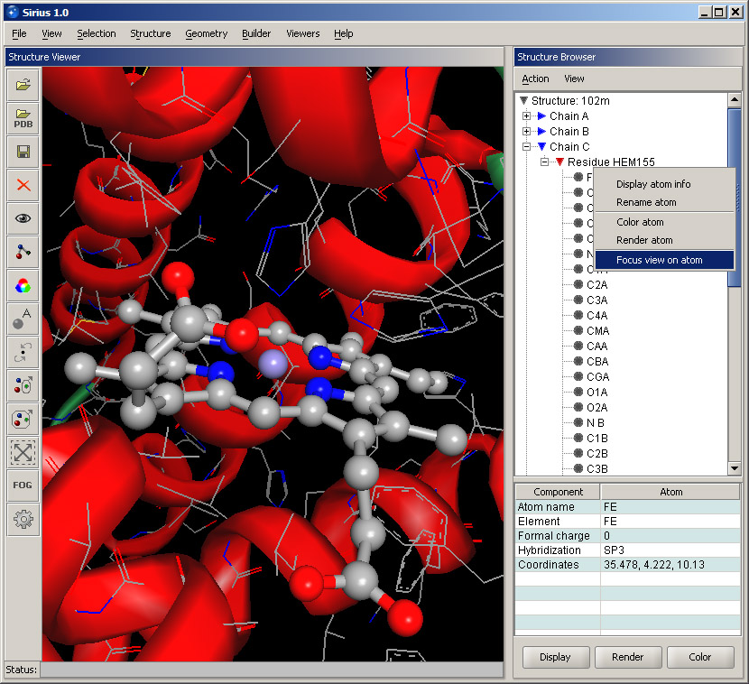
You can further focus on the ligand: expand the ligand residue by clicking its "+" sign, and its list of atoms will appear. Right-click on the FE atom and select Focus view on atom. This will bring the ligand into a close view. Note that the ribbon will appear rough and not well rendered at this zoom level. The appearance can be significantly improved by using a higher quality setting in the ribbon display dialog.

The shortcut menu also provides basic appearance commands that you can use to change rendering or color of the atom. The same applies to similar menus for residues and chains shown within the Structure Browser.

Step 4

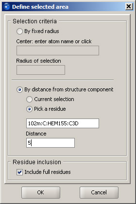
Zoom out to bring more of the protein structure into view. It may be useful to adjust the fog settings to create a better feel of depth in the display (see above).

In order to highlight protein residues that are in contact with the ligand, use option Define selection area in the Selection menu. This function can select residues within a certain radius from a given atom, but we will use a different option: selection By distance from structure component. After selecting this option, click Pick a residue and click the ligand in the 3D window. In the distance field, enter 5 (five angstroms).

Leave the option Include full residues enabled. It will ensure that full residues will be selected, as long as at least one atom is within the specified distance from the ligand.

Click OK. The residues and the corresponding fragments of the ribbon that are within 5 angstroms from the heme are highlighted.

Next, right click on the Chain A line in the Structure Browser and select Remove ribbon. This shortcut menu is the easiest method for displaying and removing a ribbon, although it does not allow for quality modification, but only adds or removes a ribbon for the corresponding chain.

Step 5

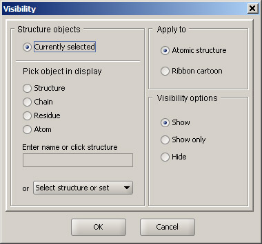
Without removing the selection (do not click anywhere in the blank area of the 3D window), hold Control key and click Chain C in the Structure Browser. This will add the heme to the current selection.

Then, select Visibility option in the View menu. Leave Currently selected option active and choose Show only in the Visibility options panel. This will hide everything except the selected part of the structure. Option Atomic structure in the Apply to section means that the operation is applied to the structure, rather than to the ribbon cartoon.

Click OK. Then click anywhere in the 3D display. The only part of the structure shown will be the heme and the surrounding residues. The view should be similar to the one shown below.

Experiment with selecting different atoms in the heme residue in the Structure Browser and note that the correspongding atoms in the 3D display are highlighted as well. Also, experiment with different colors applied to residues around the heme by using the shortcut menus and their color options. Remember that the surrounding residues belong to Chain A.

Step 6

Remove the loaded structure from the viewer by selecting Close all entries or Close entry -> 102m in the File menu of the main window. In the Viewers menu, select option Sequence Viewer. This will open a new panel at the bottom of the window. Hide Structure Browser by unchecking its check box in the Viewers menu.

Next, you will align two protein structures. Load two proteins from the Protein Data Bank: 1HCK and 1STC. Along with the structures, you will see primary sequences of the proteins in the Sequence Viewer. The sequences can be scrolled using the bar at the bottom of the panel.

Create a ribbon for each protein using Protein ribbon display option in the View menu. Since the two protein structures were determined in different conditions by different groups, they are in different coordinate systems. Therefore, once the second structure is loaded, they appear far apart in space.

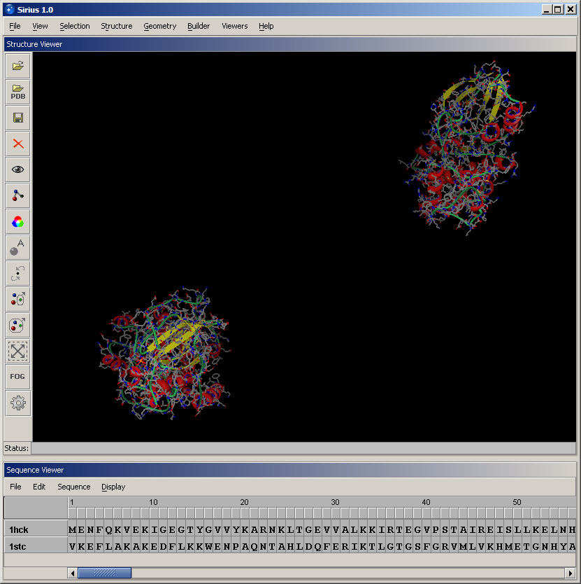
Next, hide the atomic structure of each protein to make the display more clear. Open Visibility dialog in the View menu, in Apply to section select 1hck from the pulldown menu, choose Hide in the Visibility options and click OK. Then repeat these steps for 1STC.

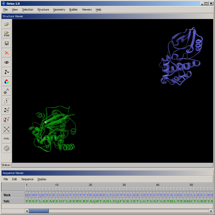
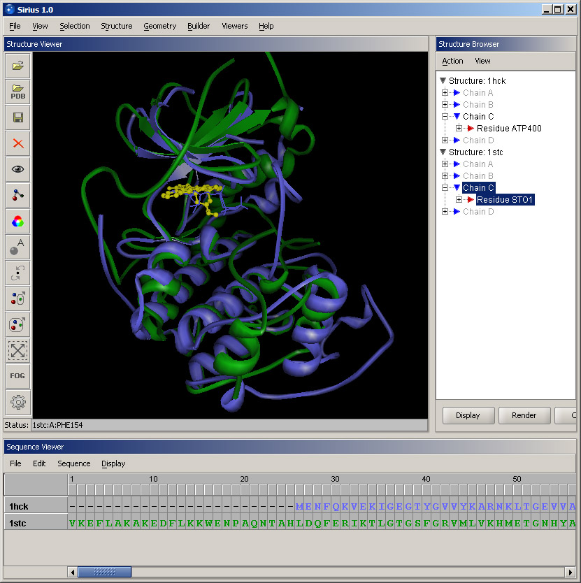
Open Color dialog under View menu and color 1HCK blue, and then 1STC green. The display should look similar to the screenshot below.

Select option Protein structure alignment in the Structure menu. In the First structure panel, select 1hck, and in the Second structure, choose 1stc. This order means that 1stc will remain in place, and coordinates of atoms of 1hck will be changed in order to align the structures.

Alternatively, structures can be picked in the 3D workspace, but selecting loaded structures from puldown menus is normally faster.

Click OK and allow a few seconds for the alignment to complete. Since there is a substantial computation involved, it may take from several seconds to a minute, depending on the processor speed.

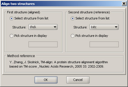
Once the calculation has completed, you can rotate the aligned structures to see which parts have aligned the best. In this case, it's several helices and a set of beta-strands. Also, take note of the sequence alignment, which was updated in the Sequence Viewer to reflect the alignment of the structures.

Open Structure Browser. Note that all chains are grayed out, which indicates that they are hidden from the view. Expand Chain C in 1hck. Select the residue and click Display button in the lower panel of Structure Browser. Click OK accepting all default settings. A selected ATP will appear in the binding site. Then repeat the same actions for Chain C in 1stc. The bound ligand in this structure is an organic molecule staurosporine. This overlay help better appreciate the similarity between the two proteins and the fact that both ligands bind in the same location within the general protein structure.

You can experiment with rendering the ligands and applying different colors to make them more visible.